All in One View
Content from Introduction: Single-Cell Transcriptomics in Weakly Electric Fish
Last updated on 2026-05-08 | Edit this page
Overview
Questions
- What genomic resources have been developed for weakly electric fish, and why?
- How does single-cell RNA sequencing differ from bulk RNA-seq, and why does that matter for studying the electric organ system?
- What is the integrated story linking hormones, the electric organ, sensory receptor tuning, and central corollary discharge in mormyrid fish?
- How can changes at the cellular and molecular level reshape behavior across seasonal, developmental, and evolutionary timescales?
Objectives
- Describe the genomic resources developed for weakly electric fish at the MSU Electric Fish Lab.
- Explain why single-cell transcriptomics is a transformative technique for biology and what kinds of questions it enables.
- Summarize how testosterone coordinately reshapes the electric organ, knollenorgan electroreceptor tuning, and central corollary discharge timing.
- Identify the molecular and cellular changes implicated in testosterone-induced EOD elongation in mormyrids.
- Connect the single-cell approach to open questions that motivate this module.
Introduction and Overview
The MSU Electric Fish Lab (https://efish.integrativebiology.msu.edu) has been leading efforts to develop genomic resources for weakly electric fish for the last 13 years. We started with the electric eel genome (Gallant et al. 2014, Science), and from there we’ve developed genomes for many of the major lineages of weakly electric fish — both South American (Gymnotiformes) and African (Mormyroidea). We’ve also developed techniques for genome manipulation using CRISPR/Cas9 and Tol2 transposases, though that’s out of the scope of this module!
Ask Vicky and Jason
If you’re curious about CRISPR/Cas9 and Tol2 transposase work in electric fish, ask Vicky Salazar and Jason about their efforts to develop these techniques.
A major innovation since the original genome and transcriptome sequencing has been the ability to sequence transcriptomes from individual cells. This technique was named Science magazine’s Breakthrough of the Year in 2018 (Pennisi 2018, Science 362:1344), and it has already led to incredible insights across biology:
- Neuroscience — comprehensive cell-type atlases of the mammalian brain (e.g., Tasic et al. 2018, Nature; the BRAIN Initiative Cell Census Network’s 2021 mouse primary motor cortex atlas, Nature) have replaced classical morphological taxonomies with molecular ones.
- Developmental and evolutionary biology — whole-embryo single-cell atlases of zebrafish (Wagner et al. 2018, Science; Briggs et al. 2018, Science) and Xenopus have reconstructed cellular lineages from zygote to organogenesis, while comparative cell-type atlases (reviewed in Tanay & Sebé-Pedrós 2021, Trends in Genetics) are letting us trace cell-type homology across millions of years of evolution.
- Genomics — single-cell approaches have revealed regulatory heterogeneity invisible to bulk RNA-seq, including rare cell states that drive disease progression and tissue regeneration.
We’ll be exploring this technique in this course module end-to-end — including sample preparation, bioinformatics, and data analysis.
The Story So Far
One of the great things about electric fish is that they “wear their behavior on their sleeves” — the behavior of interest, of course, is the electric organ discharge (EOD), which is used for both communication and electrolocation. The temporal properties of the EOD waveform, as well as the rate at which the electric organ fires, have considerable bearing on the day-to-day lives of these fish, as you have doubtlessly learned. What we’ll be working on for this module is a rather interesting example of integration across the nervous system, coordinated by hormones.
The peripheral story: hormones, the electric organ, and the EOD
The story begins with Bass & Hopkins (1983, Science 220:971–974), who demonstrated that mormyrids show seasonal sexual dimorphism in EOD waveform: males elongate their EODs during the breeding season — a change associated with the drop in conductivity that comes with the rainy season — while females do not. Bass and Hopkins showed that this change can be induced in the laboratory by exposure to 17α-methyltestosterone (17αMT), and that hormone treatment elicits a male-like response in females and juveniles as well.
A series of follow-up studies established what testosterone is actually doing to the electric organ:
- Structural changes (Bass, Denizot, & Marchaterre 1986; Freedman et al. 1989). The wafer-shaped electrocytes that make up the electric organ undergo dramatic remodeling under T treatment. Surface area of both the anterior and posterior faces of the electrocyte increases, but the increase is more pronounced on the anterior face, driven by the elaboration of deep membrane invaginations. Overall electrocyte width also increases.
- Physiological changes (Bass & Volman 1987, PNAS). Intracellular recordings from individual electrocytes showed that T elongates the duration of the action potentials generated by both faces of the electrocyte by 2–3×, with little effect on AP amplitude. The current model is that increased anterior-face surface area raises membrane capacitance, which delays spike initiation in the anterior face relative to the posterior face — preventing the two APs from canceling and producing a longer overall EOD.
- Sensory tuning (Bass & Hopkins 1984). Knollenorgan electroreceptors — the receptors specifically dedicated to detecting incoming EODs — also retune under hormone treatment. And wouldn’t you know it: their tuning shifts in exactly the same direction, becoming more sensitive to the lower peak frequencies that characterize long-duration EODs. So the periphery isn’t just changing the signal — it’s also retuning the receivers.
Stop and predict
Before reading the next section: if testosterone elongates a male’s EOD, and elongates the spike that knollenorgan receptors fire in response to that EOD, what would have to happen centrally in the brain to keep the fish from confusing its own (now-longer) EOD with an EOD from another fish?
The molecular layer: what we recently published
Last year, Mauricio Losilla and I published a paper (Losilla & Gallant 2025, J. Exp. Biol. 228:jeb249548) that took the next mechanistic step: what genes change expression as the EOD elongates? We used a clean experimental design — Brienomyrus brachyistius exposed to 17αMT for 1 day or 8 days versus ethanol-vehicle controls — and performed RNA-seq plus differential expression and functional enrichment analyses on caudal peduncle tissue.
By day 8, EOD duration had nearly doubled, and we identified 44 genes of highest interest whose expression tracked the elongation. They cluster into four functional themes:
- Cytoskeletal & sarcomeric — strong upregulation of actin and actin-related genes (actn1, actc1c, myh6, acta1b, xirp1, myo1d) and microtubule-related genes (eml6, tubb2, cavin4b, mid1ip1l). These are consistent with the cytoskeletal scaffolding required to support the expanded, more elaborately invaginated membrane.
- Extracellular matrix — upregulation of a collagen gene (si:dkey-61l1.4), thrombospondin thbs4b, and cadherin cdh11; downregulation of epdl2, an ependymin-related gene that we previously implicated in EOD waveform variation across Paramormyrops.
- Lipid metabolism — strong upregulation of elovl7a and selenoi (membrane-lipid biosynthesis) and fam126a (a gene with a known role in cell types with expanded plasma membrane). Increased membrane area presumably requires more phospholipid.
- Cation homeostasis — a coordinated shift in voltage-gated ion channel expression. We found one Na⁺ channel β-subunit gene (scn4b, downregulated) and five voltage-gated K⁺ channels. Four are delayed-rectifiers — kcna1 (Kv1.1), kcna7a1 (Kv1.7), kcnc1 (Kv3.1), and kcnc2 (Kv3.2) — all downregulated in long-EOD fish, which would slow K⁺ efflux and prolong APs. The fifth, kcng4a (Kv6.4), is a “modifier/silencer” subunit and is upregulated; its known effect on Kv2.1 is to shift inactivation to more negative potentials, again favoring AP elongation. Notably, the most highly expressed K⁺ channel in mormyrid electrocytes — kcna7a2 — did not change significantly, suggesting EOD elongation is modulated through coordinated regulation of several less-abundantly-expressed channels rather than the dominant one.
So the molecular picture aligns beautifully with the morphological and physiological work: the same cells are simultaneously remodeling their cytoskeleton and ECM contacts, expanding their membrane via lipid biosynthesis, and retuning their ionic currents.
Why this matters for single-cell
The Losilla & Gallant (2025) study used bulk RNA-seq on whole caudal peduncle tissue — a mixture of electrocytes, connective tissue, nerves, and skin. The signals we recovered are real, but they’re averaged across cell types. Single-cell transcriptomics promises to tell us which cells are doing what — and that’s a key motivation for this module.
The central layer: corollary discharge
Another aspect of this system that we haven’t yet discussed is the corollary discharge — something mormyrids are a famous model system for. When a mormyrid produces an EOD, the command originates in the command nucleus (CN) in the hindbrain. CN drives the medullary relay nucleus (MRN), which in turn drives spinal electromotor neurons that activate the electric organ.
Critically, CN also sends an efference copy of that command down a parallel corollary discharge (CD) pathway: CN → bulbar command-associated nucleus (BCA) → mesencephalic command-associated nucleus (MCA) → sublemniscal nucleus (slem). The slem is GABAergic and provides precisely-timed inhibition onto the adendritic neurons of the nucleus of the electrosensory lateral line lobe (nELL) — the same neurons that receive excitatory input from knollenorgan primary afferents. Because the inhibition arrives just as the knollenorgan reafferent spikes do, the fish is effectively “deaf” to its own EODs, and the downstream knollenorgan pathway is dedicated to processing EODs from other fish (Bell & Grant 1989; reviewed in Fukutomi & Carlson 2020).
What’s more, Bruce Carlson’s lab has shown that this central pathway is also hormonally sensitive — and adjusts in a way that beautifully complements the peripheral changes. Three findings are especially relevant:
- Fukutomi & Carlson (2023, Current Biology) showed that T treatment in B. brachyistius not only elongates the EOD (peripherally) but also delays and elongates the time window of CD inhibition in the brain. Critically, the timing of this shifted inhibition matches the shifted timing of knollenorgan reafferent input almost exactly — so the system continues to cleanly cancel responses to the fish’s own EOD even as the EOD changes shape.
- The shift is not driven by sensory feedback. Fukutomi & Carlson surgically silenced fish (spinal cord transection) so that T elongated electrocyte properties without producing any actual EODs, and then measured CD timing. The CD shift still occurred. So testosterone is acting directly on the central CD circuit, not adjusting it via altered reafference.
- Jarzyna & Carlson (2026, preprint) then localized the central effect: simultaneous field-potential recordings throughout the CD pathway show that the shift in onset and duration of CD activity originates at the mesencephalic command-associated nucleus (MCA), propagating through slem to nELL. Even more elegantly, the same MCA locus accounts for evolutionary differences between short-EOD (C. compressirostris) and long-EOD (C. numenius) species, and for developmental plasticity in extreme long-EOD adult C. numenius. So one neural substrate handles seasonal hormonal shifts (days), developmental shifts (years), and evolutionary divergence (millions of years).
That last point is what makes this such a satisfying integration story: from a single hormonal cue, the periphery (electric organ) and the central nervous system (corollary discharge circuitry) are co-regulated to keep the entire sensorimotor loop coherent. And the central locus appears to be reused across timescales of plasticity. This is the system we’ll be probing at single-cell resolution in this module.
Putting it together
Sketch the loop linking testosterone, the electric organ, knollenorgan electroreceptors, and the corollary discharge pathway. For each component, note one thing that changes under T treatment and one outstanding question that single-cell transcriptomics could address.
Possible answers (yours may differ — the goal is to make the integration explicit):
- Electric organ / electrocytes — change: anterior-face surface area expands, K⁺/Na⁺ channel expression shifts, cytoskeleton remodels. Open question: are these changes uniform across all electrocytes, or are there electrocyte sub-populations responding differently?
- Knollenorgan electroreceptors — change: tuning shifts to lower peak frequency. Open question: is this driven by a single cell-type-specific transcriptional program, and is the same program triggered by T as in the electric organ?
- CD pathway (especially MCA) — change: onset and duration of CD activity is delayed and elongated to match shifted reafferent input. Open question: which cell types in MCA express androgen / estrogen receptors, and is the same molecular toolkit used here as in the periphery?
- Loop integration — change: the entire sensorimotor loop stays internally consistent across seasons, development, and species. Open question: what shared molecular signatures define cell types that are “T-responsive” across this whole circuit?
Key references
Pennisi, E. (2018). Development cell by cell. Science 362:1344 [Breakthrough of the Year].
- The MSU Electric Fish Lab has built genomic resources spanning the major weakly electric fish lineages, beginning with the electric eel genome in 2014.
- Single-cell RNA-seq (named Science’s Breakthrough of the Year in 2018) reveals cell-type-specific biology that bulk RNA-seq cannot resolve.
- In mormyrids, testosterone elongates the EOD by remodeling electrocyte morphology and physiology, retunes knollenorgan electroreceptors, and shifts central corollary discharge timing — all coordinated to keep the sensorimotor loop coherent.
- The Losilla & Gallant (2025) paper identified 44 genes of interest, including cytoskeletal, ECM, lipid-metabolism, and ion channel genes — but bulk RNA-seq cannot tell us which cell types drive these signals.
- The same neural locus (MCA) appears to handle seasonal, developmental, and evolutionary shifts in CD timing — a striking example of substrate reuse across timescales.
- Single-cell transcriptomics is the natural next step to ask which cells in this integrated system carry which molecular signatures of plasticity.
Content from 11-Ketotestosterone Implantation in Mormyrid Electric Fish
Last updated on 2026-05-08 | Edit this page
Background
Cocoa butter melts at body temperature, which makes it a useful slow-release vehicle for lipophilic steroids implanted into the peritoneal cavity. Bass and colleagues established this approach in the 1980s for studies of androgen action on the electric organ in mormyrids (Bass et al., 1986; Bass et al., 1987). A single 20% w/w cocoa-butter implant of 11-KT yields elevated circulating androgen for several days and produces measurable shifts in EOD waveform within ~24–72 h, depending on species and dose.
This episode walks through the Day 0 implant procedure as it is run in our lab. It assumes that the broader experimental schedule (acclimation, weighing, tank assignment, post-implant recording cadence) is already defined elsewhere in the course materials.
Why cocoa butter?
Cocoa butter is solid at room temperature, liquefies at 35–40 °C, and re-solidifies inside the fish — trapping the steroid in a slow-release depot. It is also non-reactive in the IP cavity and avoids the need for a DMSO/oil carrier injection.
Reagents
- Cocoa butter chips
- 11-KT (Steraloids A6720, 25 mg vial)
- MS-222 (tricaine methanesulfonate)
- Vetbond (tissue adhesive)
- Recovery water (system water with NaCl supplement)
- Maintenance-dose MS-222 (for gill drip during surgery, if used)
Equipment
- Scalpel (sharp, fresh blade)
- Kimwipes
- Dry bath
- Milligram balance
- P200 pipette + tips
- Dissecting tray + dissecting pins
- Recovery containers
- Fish-transfer net
Step 0: EOD baseline (Day −1 and Day 0, pre-implant)
- Record an EOD waveform from each fish on Day −1 (24 h prior) and again on Day 0 immediately before implantation. These pre-treatment recordings are the per-fish baselines that all post-implant measurements will be normalized to (Bass et al., 1986).
- Confirm fish ID, weight, and tank assignment are logged before proceeding to Step 1.
Why two baselines?
Day −1 captures the fish’s “settled” waveform; Day 0 confirms it has not drifted overnight. If the two recordings disagree by more than your normal day-to-day variability, do not implant — investigate first.
Step 1: Prepare 11-KT doses (20% w/w in cocoa butter)
- Melt 1 cocoa-butter chip (≈ 1.75 mL) at 40 °C.
- Weigh out 6.5 mg 11-KT.
- Combine the 11-KT with 35 µL of melted cocoa butter and pipette up and down thoroughly while maintaining heat at 35–40 °C, until 11-KT crystals are fully dissolved and the solution appears clear/translucent. If particles persist after 2 min at temperature, hold longer before pipetting.
- Keep the dose mix on the dry bath until ready for implantation.
Don’t rush dissolution
11-KT does dissolve fully in cocoa butter at this loading and temperature, but it isn’t instantaneous. Pipetting before the crystals are gone gives non-uniform doses across your fish — the first fish gets a heavy bolus, the last gets diluted vehicle.
Calculating the dose
You want to implant 5 fish at 1 mg 11-KT per dose, with ~30% extra prep volume to absorb pipetting losses. Working at 20% w/w, how much 11-KT do you weigh out, and how much cocoa butter do you combine it with?
- Per-dose 11-KT mass: 1 mg.
- For 5 fish + 30%: ≈ 6.5 mg of 11-KT.
- At 20% w/w, the matching cocoa-butter mass is ≈ 26 mg, which corresponds to roughly 35 µL of melted cocoa butter (density ≈ 0.9 g/mL).
This is the recipe used in Step 1 above.
Step 2: Anesthetize fish & sterilize equipment
- Anesthetize the fish in MS-222 (0.1–0.2 g/L) until it loses its righting response but is still actively gilling.
- Spray tools with 70% ethanol and let sit for 5 minutes, then dry with a kimwipe. Alternatively, use a heat sterilizer — just make sure the tools are properly cooled before they touch the fish.
Surgical plane, not deep anesthesia
You want gilling to continue throughout the procedure. If gill movement stops, you have gone too deep — move the fish into fresh water immediately.
Step 3: Implantation of 11-KT
- Remove the fish from the anesthetic and place it in the dissecting tray, belly-up, leaning against two dissecting pins.
- Blot the surgical area dry with a kimwipe.
- With a sharp, fresh scalpel blade, make a small incision anterior to the anal pore and slightly off the ventral midline (to avoid major vessels), passing through skin and muscle wall into the peritoneal cavity. The cut should be just wide enough to fit a P200 pipette tip, and should feel “deep” enough that you are clearly through the muscle wall.
- Draw 5 µL of the 11-KT / cocoa-butter mix from the heated solution and immediately deposit it through the incision. A successful implantation leaves all material deep within the cut, not on the surface.
- If any blood or fluid is on the outside of the fish, blot once more with a kimwipe.
- Apply a small amount of Vetbond over the incision and wait for it to skin, checking that the seal is complete. Apply more Vetbond if necessary, but take care that it is not “wicked” onto the pectoral fins or gills nearby.
- Place the fish into fresh recovery water and wait ~20 minutes for it to return upright before returning it to its home tank.
Incision location matters
Bass’s original phrasing was “small incision was made anterior to the anal pore.” Going off-midline keeps you out of the major ventral vessels, and staying anterior to the anal pore puts the dose into the IP cavity proper rather than the cloacal region.
Troubleshooting a failed seal
Five minutes after implantation you notice a small bead of cocoa-butter / 11-KT solution sitting on the fish’s belly, outside the Vetbond. What do you do, and how do you note it in the experimental log?
- Blot the surface dose off with a fresh kimwipe.
- Apply a second layer of Vetbond and let it skin.
- Note the partial extrusion in the log: dose delivered is uncertain. This animal should be flagged for exclusion or, at minimum, tracked separately when EOD changes are analyzed — the slow-release pharmacology assumes the depot is fully internal.
After surgery
Once each fish is upright and swimming, return it to its labeled home tank and resume the post-implant EOD recording schedule defined in the broader course protocol. Do not feed for 24 h.
- Cocoa-butter implants give a several-day, slow-release androgen exposure with a single Day 0 procedure.
- Pre-treatment EOD recordings on Day −1 and Day 0 are the per-fish baselines — every post-implant measurement is interpreted relative to them.
- Full dissolution of 11-KT in warm cocoa butter is what makes the dose uniform across animals; rushing this step is the most common avoidable source of variance.
- Incise anterior to the anal pore, slightly off the ventral midline, and seal cleanly with Vetbond.
- A surface-extruded dose is not a delivered dose — flag the animal in the log.
References
- Bass, A. H., et al. (1986). Androgen binding in the brain and electric organ of a mormyrid fish.
- Bass, A. H., et al. (1987). From behavior to membranes: testosterone-induced changes in action potential duration in electric organs.
Content from Examining EOD Duration from Raw Recordings
Last updated on 2026-05-08 | Edit this page
Overview
Questions
- How do we load JSON EOD recordings into R?
- How is EOD duration measured from a raw waveform?
- Did 11-ketotestosterone treatment change EOD duration over time?
Objectives
- Load JSON recording files into R using the
jsonlitepackage - Navigate a list of recording objects to extract waveform data and metadata
- Visualize a raw EOD waveform using
ggplot2 - Measure EOD duration by applying a threshold to a normalized waveform
- Build a tidy dataset by applying a duration function across many files
- Check ANOVA assumptions using Levene’s and Shapiro-Wilk tests
- Perform a one-way ANOVA and interpret the result
- Interpret a faceted comparison plot of EOD duration across treatment groups
Introduction
In the previous episodes, you learned how testosterone shapes the electric organ discharge (EOD) in Brienomyrus brachyistius, and you performed the implantation procedure yourself. Now it’s time to analyze the data.
EOD recordings were captured daily over 8 days for animals implanted with either 11-ketotestosterone (11-kt) or a blank control. Each recording session is stored as a JSON file containing multiple trials. Our goal is to:
- Load a raw EOD waveform and visualize it
- Write a function that measures EOD duration from any recording file
- Apply that function across all recording sessions to build a dataset
- Test whether 11-kt treatment changed EOD duration over time
Loading EOD Recording Files in R
JSON files can be read in R using the jsonlite package.
The read_json() function returns a list that maps directly
onto the file structure.
R
library(jsonlite)

eod_data <- read_json("data/eod_duration/DAY0_MAY5/BB_T48.json")

cat("Number of recordings:", length(eod_data), "\n")
OUTPUT
Number of recordings: 11 Each element of eod_data is one recording trial, stored
as a named list. Use names(eod_data[[1]]) to see the
available fields and $ to access them.
Challenge 1: Explore the recording metadata (5 min)
Using the eod_data object already loaded, print the
specimen number, species, temperature, sampling rate, and number of
waveform samples for the first recording trial.
Hint: names(eod_data[[1]]) shows the available
fields.
R
names(eod_data[[1]])
cat("Specimen:", eod_data[[1]]$specimenno, "\n")
cat("Species: ", eod_data[[1]]$species, "\n")
cat("Temp:    ", eod_data[[1]]$temp, "\n")
cat("Rate:    ", eod_data[[1]]$Rate, "\n")
cat("Samples: ", length(eod_data[[1]]$wave), "\n")
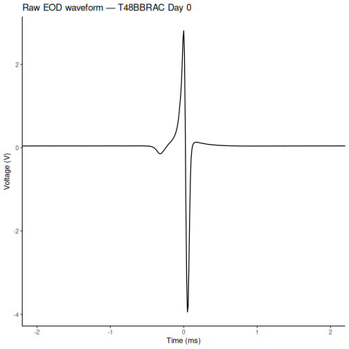
Visualizing an EOD Waveform
We convert sample indices to milliseconds using the sampling rate
stored in the file, then plot with ggplot2.
R
library(ggplot2)

rate_hz <- eod_data[[1]]$Rate
wave    <- unlist(eod_data[[1]]$wave)
p1_idx  <- which.max(wave)
time_ms <- (seq_along(wave) - p1_idx) / rate_hz * 1000

waveform_df <- data.frame(time_ms = time_ms, voltage = wave)

ggplot(waveform_df, aes(x = time_ms, y = voltage)) +
  geom_line(linewidth = 0.6) +
  coord_cartesian(xlim = c(-2, 2)) +
  theme_classic() +
  labs(
    x = "Time (ms)",
    y = "Voltage (V)",
    title = paste("Raw EOD waveform —", eod_data[[1]]$specimenno, "Day 0")
  )
Challenge 2: Compare waveforms across recording sessions (5 min)
Load the first recording from
data/eod_duration/DAY0_MAY7/BBRAC_T48_MAY7.json and plot it
alongside the May 5 waveform. Do the shapes look similar?
R
eod_may7  <- read_json("data/eod_duration/DAY0_MAY7/BBRAC_T48_MAY7.json")
wave7     <- unlist(eod_may7[[1]]$wave)
p1_idx7   <- which.max(wave7)
time7_ms  <- (seq_along(wave7) - p1_idx7) / eod_may7[[1]]$Rate * 1000

df_compare <- rbind(
  data.frame(time_ms = time_ms,  voltage = wave,  session = "May 5"),
  data.frame(time_ms = time7_ms, voltage = wave7, session = "May 7")
)

ggplot(df_compare, aes(x = time_ms, y = voltage, color = session)) +
  geom_line(linewidth = 0.6) +
  coord_cartesian(xlim = c(-2, 2)) +
  theme_classic() +
  scale_colour_manual(values = c("May 5" = "grey50", "May 7" = "tomato")) +
  labs(x = "Time (ms)", y = "Voltage (V)",
       title = "Day 0 EOD waveforms — two recording sessions",
       color = NULL)
Both are Day 0 baseline recordings taken before any treatment, so the waveform shapes should be similar.
Measuring EOD Duration
EOD duration is not read directly from the file — it must be calculated from the waveform. The standard approach is:
- Normalize the waveform so that the peak-to-peak amplitude = 1
- Apply a threshold (typically 10% of the maximum absolute value) to define where the EOD “starts” and “ends”
- Calculate duration as the time elapsed between the first and last threshold crossings
R
# 1. Normalize to peak-to-peak = 1
wave_norm <- wave / (max(wave) - min(wave))

# 2. Apply 10% threshold
threshold    <- 0.1 * max(abs(wave_norm))
above_thresh <- which(abs(wave_norm) > threshold)

start_idx <- min(above_thresh)
end_idx   <- max(above_thresh)

# 3. Duration in milliseconds
duration_ms <- (end_idx - start_idx) / rate_hz * 1000
cat("EOD duration (10% threshold):", round(duration_ms, 3), "ms\n")
OUTPUT
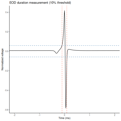
EOD duration (10% threshold): 0.19 msWe can visualize the threshold on the normalized waveform to see exactly which part of the signal is being measured:
R
norm_df <- data.frame(time_ms = time_ms, voltage = wave_norm)

ggplot(norm_df, aes(x = time_ms, y = voltage)) +
  geom_line(linewidth = 0.6) +
  geom_hline(yintercept = c(threshold, -threshold),
             linetype = "dashed", color = "steelblue", linewidth = 0.5) +
  geom_vline(xintercept = c(time_ms[start_idx], time_ms[end_idx]),
             linetype = "dashed", color = "tomato", linewidth = 0.5) +
  coord_cartesian(xlim = c(-2, 2)) +
  theme_classic() +
  labs(
    x     = "Time (ms)",
    y     = "Normalized voltage",
    title = "EOD duration measurement (10% threshold)"
  )
Challenge 3: Sensitivity of the threshold (5 min)
Repeat the duration calculation using a 20% threshold instead of 10%. How does the measured duration change, and why?
This is important: the choice of threshold is an analytical decision that must be reported in any publication.
R
threshold_20  <- 0.2 * max(abs(wave_norm))
above_20      <- which(abs(wave_norm) > threshold_20)

duration_20ms <- (max(above_20) - min(above_20)) / rate_hz * 1000
cat("Duration at 20% threshold:", round(duration_20ms, 3), "ms\n")
cat("Duration at 10% threshold:", round(duration_ms, 3), "ms\n")
A higher threshold excludes the low-amplitude tails of the waveform, making the measured duration shorter. Neither threshold is “wrong” — but the choice must be consistent across all animals in a study and clearly reported.
Building a Dataset Across All Recording Sessions
Now that we know how to measure EOD duration from a single file, we can apply the same logic to every recording session in the study. Rather than computing durations by hand for each file, we write a function and let R do the work.
The study metadata is stored in recordings.csv, which
maps each JSON file to its animal, day, and treatment group:
R
library(dplyr)

metadata <- read.csv("data/eod_duration/recordings.csv")
metadata$Treatment <- as.factor(metadata$Treatment)

head(metadata)
OUTPUT
                           file specimenno day Treatment
1         DAY0_MAY5/BB_T48.json       BB48   0     11-kt
2         DAY0_MAY5/BB_T49.json       BB49   0     11-kt
3         DAY0_MAY5/BB_T50.json       BB50   0   control
4         DAY0_MAY5/BB_T51.json       BB51   0   control
5 DAY0_MAY7/BBRAC_T48_MAY7.json       BB48   1     11-kt
6 DAY0_MAY7/BBRAC_T49_MAY7.json       BB49   1     11-kt
We write a small function that takes a file path, loads the JSON, computes EOD duration for every trial, and returns the mean:
R
mean_eod_duration <- function(file_path, threshold = 0.1) {
  recs <- read_json(file_path)
  durations <- sapply(recs, function(rec) {
    w      <- unlist(rec$wave)
    rate   <- rec$Rate
    w_norm <- w / (max(w) - min(w))
    thresh <- threshold * max(abs(w_norm))
    above  <- which(abs(w_norm) > thresh)
    (max(above) - min(above)) / rate * 1000
  })
  mean(durations)
}
We then apply this function to every row in the metadata table:
R
metadata$EOD <- sapply(
  file.path("data/eod_duration", metadata$file),
  mean_eod_duration
)

head(metadata)
OUTPUT
file specimenno day Treatment EOD
1 DAY0_MAY5/BB_T48.json BB48 0 11-kt 0.1900000
2 DAY0_MAY5/BB_T49.json BB49 0 11-kt 0.2260000
3 DAY0_MAY5/BB_T50.json BB50 0 control 0.1900000
4 DAY0_MAY5/BB_T51.json BB51 0 control 0.1900000
5 DAY0_MAY7/BBRAC_T48_MAY7.json BB48 1 11-kt 0.2472727
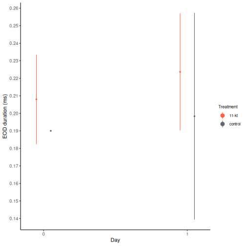
6 DAY0_MAY7/BBRAC_T49_MAY7.json BB49 1 11-kt 0.2000000Longitudinal trajectory
With the full dataset assembled, we can visualize how EOD duration changes across the 8-day experiment for each treatment group. Points show the group mean; error bars show ±1 standard deviation.
R
ggplot(metadata, aes(x = day, y = EOD, group = Treatment, color = Treatment)) +
  stat_summary(
    fun     = "mean",
    geom    = "pointrange",
    fun.max = function(x) mean(x) + sd(x),
    fun.min = function(x) mean(x) - sd(x),
    position = position_dodge(width = 0.2, preserve = "total"),
    size    = 0.7,
    fatten  = 0.5
  ) +
  scale_x_continuous(name = "Day", breaks = 0:8) +
  scale_y_continuous(
    name   = "EOD duration (ms)",
    breaks = scales::breaks_pretty(10)
  ) +
  scale_colour_manual(values = c("11-kt" = "tomato", "control" = "grey40")) +
  theme_classic() +
  theme(
    axis.text    = element_text(size = 9),
    legend.text  = element_text(size = 8),
    legend.title = element_text(size = 9)
  )
Testing assumptions
Before running an ANOVA, we verify two key assumptions:
-
Homogeneity of variance — tested with Levene’s test
(
car::leveneTest) - Normality of residuals — tested with the Shapiro-Wilk test
R
suppressPackageStartupMessages(library(car))

# Extract Day 0 baseline data
d0 <- metadata %>% filter(day == 0)

res_aov_d0 <- aov(EOD ~ Treatment, data = d0)

lev_d0 <- leveneTest(res_aov_d0)
print(lev_d0)
OUTPUT
Levene's Test for Homogeneity of Variance (center = median)
      Df    F value    Pr(>F)
group  1 2.9908e+30 < 2.2e-16 ***
       2
---
Signif. codes:  0 '***' 0.001 '**' 0.01 '*' 0.05 '.' 0.1 ' ' 1
R
shp_d0 <- shapiro.test(residuals(res_aov_d0))
print(shp_d0)
OUTPUT
	Shapiro-Wilk normality test

data:  residuals(res_aov_d0)
W = 0.94466, p-value = 0.683
If neither test is significant (p > 0.05), the ANOVA assumptions are met.
Challenge 4: Full statistical comparison (10 min)
Work through the following steps:
Step 1. Inspect the Day 0 ANOVA — do the treatment groups differ at baseline?
R
summary(res_aov_d0)
Step 2. Extract Day 8 data and run the same ANOVA. Check assumptions first.
R
d8 <- metadata %>% filter(day == 8)

res_aov_d8 <- aov(EOD ~ Treatment, data = d8)

leveneTest(res_aov_d8)
shapiro.test(residuals(res_aov_d8))

summary(res_aov_d8)
Step 3 (stretch). Reproduce the faceted plot below, showing Day 0 and Day 8 distributions side by side with individual data points overlaid.
R
# Step 1 — baseline check
summary(res_aov_d0)
# Non-significant: groups were similar before treatment.

# Step 2 — end-of-treatment comparison
d8 <- metadata %>% filter(day == 8)
res_aov_d8 <- aov(EOD ~ Treatment, data = d8)
leveneTest(res_aov_d8)
shapiro.test(residuals(res_aov_d8))
summary(res_aov_d8)

# Step 3 — faceted plot
d_plot <- bind_rows(
  mutate(d0, timepoint = "Day 0"),
  mutate(d8, timepoint = "Day 8")
)

ggplot(d_plot, aes(x = Treatment, y = EOD, color = Treatment)) +
  stat_summary(
    fun     = "mean",
    geom    = "pointrange",
    fun.max = function(x) mean(x) + sd(x),
    fun.min = function(x) mean(x) - sd(x),
    fatten  = 1.8
  ) +
  geom_point(shape = 2, position = position_jitter(width = 0.07, seed = 84)) +
  facet_wrap(~timepoint) +
  scale_y_continuous(
    name   = "EOD duration (ms)",
    breaks = scales::breaks_pretty(10)
  ) +
  scale_colour_manual(values = c("11-kt" = "tomato", "control" = "grey40")) +
  theme_classic() +
  theme(
    axis.text       = element_text(size = 9),
    legend.position = "none",
    panel.border    = element_rect(colour = "black", fill = NA)
  )
-
jsonlite::read_json()loads JSON files as nested R lists; each recording trial is a named list with fields likewave,Rate,temp, andspecimenno - EOD duration is defined by a threshold criterion applied to the normalized waveform — the choice of threshold is an analytical decision that must be reported
- A metadata CSV that maps files to experimental conditions lets you build a tidy dataset by applying a duration function across all recording sessions
- Always verify ANOVA assumptions (Levene’s test for equal variance; Shapiro-Wilk on residuals for normality) before interpreting results